如果你也在 怎样代写回归分析Regression Analysis 这个学科遇到相关的难题,请随时右上角联系我们的24/7代写客服。回归分析Regression Analysis回归中的概率观点具体体现在给定X数据的特定固定值的Y数据的可变性模型中。这种可变性是用条件分布建模的;因此,副标题是:“条件分布方法”。回归的整个主题都是用条件分布来表达的;这种观点统一了不同的方法,如经典回归、方差分析、泊松回归、逻辑回归、异方差回归、分位数回归、名义Y数据模型、因果模型、神经网络回归和树回归。所有这些都可以方便地用给定特定X值的Y条件分布模型来看待。
回归分析Regression Analysis条件分布是回归数据的正确模型。它们告诉你,对于变量X的给定值,可能存在可观察到的变量Y的分布。如果你碰巧知道这个分布,那么你就知道了你可能知道的关于响应变量Y的所有信息,因为它与预测变量X的给定值有关。与基于R^2统计量的典型回归方法不同,该模型解释了100%的潜在可观察到的Y数据,后者只解释了Y数据的一小部分,而且在假设几乎总是被违反的情况下也是不正确的。
回归分析Regression Analysis代写,免费提交作业要求, 满意后付款,成绩80\%以下全额退款,安全省心无顾虑。专业硕 博写手团队,所有订单可靠准时,保证 100% 原创。 最高质量的回归分析Regression Analysis作业代写,服务覆盖北美、欧洲、澳洲等 国家。 在代写价格方面,考虑到同学们的经济条件,在保障代写质量的前提下,我们为客户提供最合理的价格。 由于作业种类很多,同时其中的大部分作业在字数上都没有具体要求,因此回归分析Regression Analysis作业代写的价格不固定。通常在专家查看完作业要求之后会给出报价。作业难度和截止日期对价格也有很大的影响。
同学们在留学期间,都对各式各样的作业考试很是头疼,如果你无从下手,不如考虑my-assignmentexpert™!
my-assignmentexpert™提供最专业的一站式服务:Essay代写,Dissertation代写,Assignment代写,Paper代写,Proposal代写,Proposal代写,Literature Review代写,Online Course,Exam代考等等。my-assignmentexpert™专注为留学生提供Essay代写服务,拥有各个专业的博硕教师团队帮您代写,免费修改及辅导,保证成果完成的效率和质量。同时有多家检测平台帐号,包括Turnitin高级账户,检测论文不会留痕,写好后检测修改,放心可靠,经得起任何考验!
统计代写|回归分析代写Regression Analysis代考|Measurement Error
Very often, the variables $X$ and $Y$ that you might use are imperfectly measured. For example, you might wish to assess the effect of a company’s accounting mistakes on their performance, but people do not like to admit mistakes, and also people might not even know that they have made mistakes. Thus, you cannot measure “Accounting Mistakes” directly. Instead, you decide to use a proxy variable, such as $X=$ CEO’s Guess of Accounting Mistakes. Clearly, the CEO’s guess is not the same as the actual number of mistakes, but they should be correlated.
Letting $X_A=$ Actual Mistakes and $X_G=C E O$ ‘s Guess, it should be clear that the conditional distribution $p\left(y \mid X_G=x\right)$ is different from the conditional distribution $p\left(y \mid X_A=x\right)$, simply because $X_G$ and $X_A$ are different variables. The results of the previous section show that the OLS estimates based on the data $\left(X_G, Y\right)$ give unbiased estimates for the model $\boldsymbol{Y}=\mathbf{X}_G \boldsymbol{\beta}_G+\boldsymbol{\varepsilon}_G$ (under the Gauss-Markov assumptions), and that the OLS estimates based on the data $\left(X_A, Y\right)$ give unbiased estimates for the model $\boldsymbol{Y}=\mathbf{X}_A \boldsymbol{\beta}_A+\boldsymbol{\varepsilon}_A$ (again, under the Gauss-Markov assumptions). However, it should be no surprise that the data $\left(X_G, Y\right)$ give biased estimates for the model $\boldsymbol{Y}=\mathbf{X}_A \boldsymbol{\beta}_A+\boldsymbol{\varepsilon}_A$, simply because $\boldsymbol{\beta}_G$ and $\boldsymbol{\beta}_A$ are different. Usually, the effect of this bias is toward zero; that is, the estimated effect (slope) based on $\left(X_G, Y\right)$ will be closer to zero, the $R^2$ statistic will be smaller, and the $p$-value larger than when you use $\left(X_A, Y\right)$.
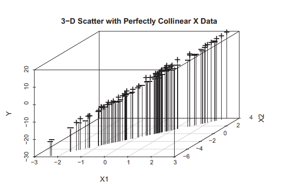
The following simulation illustrates this bias in the case where the $X_A$ variable is “Widgets” and the $X_G$ variable is a guess at the number of Widgets, e.g., by a plant supervisor. The simulation assumes that $X_G$ differs from $X_A$ by random error, with $X_G=X_A+\delta$. The term $\delta$ is called the “measurement error,” and is assumed to be independent of $X_A$ and $\varepsilon_A$. The code is similar to the code that produced Figure 7.2 above, but with the addition of normally distributed measurement error $\delta$.
统计代写|回归分析代写Regression Analysis代考|Standard Errors of OLS Estimates
Recall from Section 3.5 that the conditional (on $\mathbf{X}=\mathbf{x}$ ) variance of $\hat{\beta}_1$ is, in the case of simple regression where there is only one $X$ variable, given by
$$
\operatorname{Var}\left(\hat{\beta}_1 \mid \mathbf{X}=\mathbf{x}\right)=\frac{\sigma^2}{(n-1) s_x^2}
$$
Taking the square root gives you the conditional standard deviation, and replacing $\sigma$ with $\hat{\sigma}$ gives you the standard error:
$$
\text { s.e. }\left(\hat{\boldsymbol{\beta}}_1 \mid \mathbf{X}=\mathbf{x}\right)=\frac{\hat{\sigma}}{s_x \sqrt{n-1}}
$$
Usually, the $\mathbf{X}=\mathbf{x}$ condition is not displayed explicitly, but clearly this standard error formula is conditional on the observed values of $\mathbf{X}$ because there is a sample estimate, $s_x$, in the formula.
In multiple regression where there is more than one $X$ variable, the standard error formula cannot be displayed in such a simple form. Matrix methods are needed instead. To get these standard errors, we first need the variance of an estimated $\beta$. Strangely, it turns out that it is easier to compute the entire covariance matrix of the estimated vector $\hat{\boldsymbol{\beta}}$, then pick the variances out from the diagonal elements of the covariance matrix. To do this, we need to invoke a famous result, a generalization of the “linearity property of variance” to covariance matrices. The result is as follows:
Linearity property of covariance matrices
Let $\boldsymbol{W}$ be a random $(p \times 1)$ vector and let $\mathbf{A}$ be a fixed (not random) $(q \times p)$ matrix. Then
$$
\operatorname{Cov}(\mathbf{A W})=\mathbf{A} \operatorname{Cov}(\boldsymbol{W}) \mathbf{A}^{\mathrm{T}}
$$
回归分析代写
统计代写|回归分析代写Regression Analysis代考|Measurement Error
通常,您可能使用的变量$X$和$Y$没有得到完美的度量。例如,您可能希望评估公司的会计错误对其绩效的影响,但是人们不喜欢承认错误,而且人们甚至可能不知道他们犯了错误。因此,你不能直接衡量“会计错误”。相反,您决定使用代理变量,例如$X=$ CEO对会计错误的猜测。显然,首席执行官的猜测与实际错误数量并不相同,但它们应该是相关的。
让$X_A=$实际错误和$X_G=C E O$的猜测,应该清楚的是,条件分布$p\left(y \mid X_G=x\right)$不同于条件分布$p\left(y \mid X_A=x\right)$,仅仅是因为$X_G$和$X_A$是不同的变量。上一节的结果表明,基于数据$\left(X_G, Y\right)$的OLS估计给出了模型$\boldsymbol{Y}=\mathbf{X}_G \boldsymbol{\beta}_G+\boldsymbol{\varepsilon}_G$的无偏估计(在高斯-马尔可夫假设下),并且基于数据$\left(X_A, Y\right)$的OLS估计给出了模型$\boldsymbol{Y}=\mathbf{X}_A \boldsymbol{\beta}_A+\boldsymbol{\varepsilon}_A$的无偏估计(再次,在高斯-马尔可夫假设下)。然而,数据$\left(X_G, Y\right)$对模型$\boldsymbol{Y}=\mathbf{X}_A \boldsymbol{\beta}_A+\boldsymbol{\varepsilon}_A$给出有偏差的估计并不奇怪,这仅仅是因为$\boldsymbol{\beta}_G$和$\boldsymbol{\beta}_A$是不同的。通常,这种偏差的影响趋向于零;也就是说,基于$\left(X_G, Y\right)$的估计效果(斜率)将更接近于零,$R^2$统计量将更小,而$p$ -值将比使用$\left(X_A, Y\right)$时更大。
下面的模拟说明了这种偏差,其中$X_A$变量是“Widgets”,$X_G$变量是对Widgets数量的猜测,例如,由工厂主管进行的猜测。模拟假设$X_G$与$X_A$因随机误差而不同,其中$X_G=X_A+\delta$。术语$\delta$被称为“测量误差”,并被认为与$X_A$和$\varepsilon_A$无关。代码类似于上面产生图7.2的代码,但是增加了正态分布的测量误差$\delta$。
统计代写|回归分析代写Regression Analysis代考|Standard Errors of OLS Estimates
回想一下第3.5节,$\hat{\beta}_1$的条件(在$\mathbf{X}=\mathbf{x}$上)方差是,在简单回归的情况下,只有一个$X$变量,由
$$
\operatorname{Var}\left(\hat{\beta}_1 \mid \mathbf{X}=\mathbf{x}\right)=\frac{\sigma^2}{(n-1) s_x^2}
$$
取平方根得到条件标准差,用$\hat{\sigma}$代替$\sigma$得到标准误差:
$$
\text { s.e. }\left(\hat{\boldsymbol{\beta}}_1 \mid \mathbf{X}=\mathbf{x}\right)=\frac{\hat{\sigma}}{s_x \sqrt{n-1}}
$$
通常,$\mathbf{X}=\mathbf{x}$条件不会显式显示,但很明显,这个标准误差公式是以$\mathbf{X}$的观测值为条件的,因为公式中有一个样本估计值$s_x$。
在多元回归中,当存在多个$X$变量时,标准误差公式不能以如此简单的形式显示。而需要矩阵方法。为了得到这些标准误差,我们首先需要估计$\beta$的方差。奇怪的是,计算估计向量$\hat{\boldsymbol{\beta}}$的整个协方差矩阵更容易,然后从协方差矩阵的对角线元素中选出方差。要做到这一点,我们需要调用一个著名的结果,将“方差的线性性质”推广到协方差矩阵。结果如下:
协方差矩阵的线性性质
设$\boldsymbol{W}$是一个随机的$(p \times 1)$向量,$\mathbf{A}$是一个固定的(不是随机的)$(q \times p)$矩阵。然后
$$
\operatorname{Cov}(\mathbf{A W})=\mathbf{A} \operatorname{Cov}(\boldsymbol{W}) \mathbf{A}^{\mathrm{T}}
$$

统计代写|回归分析代写Regression Analysis代考 请认准UprivateTA™. UprivateTA™为您的留学生涯保驾护航。